Time Series Analysis
Time series objects deserve a special mention as they can be useful for numerical data and allow the ability to forecast which can be useful for example when determining what the throughput in an outpatient clinic is likely to be so we can plan ahead.
Create a time series- numerical data
Dataframes can be formatted as time series objects as follows
#Sample dates
dat<-sample(seq(as.Date('2013/01/01'), as.Date('2017/05/01'), by="day"), 100)

rndm1<-sample(seq(0,40),100,replace=T)
rndm2<-sample(seq(0,40),100,replace=T)
rndm3<-sample(seq(0,40),100,replace=T)
df<-data.frame(dat,rndm1,rndm2,rndm3)


library(xts)
Myxts<-xts(df, order.by=df$dat)
kable(head(Myxts,25))| dat | rndm1 | rndm2 | rndm3 |
|---|---|---|---|
| 2013-01-13 | 11 | 6 | 37 |
| 2013-02-01 | 38 | 13 | 20 |
| 2013-03-20 | 32 | 1 | 15 |
| 2013-05-18 | 39 | 29 | 1 |
| 2013-05-29 | 21 | 14 | 21 |
| 2013-06-11 | 37 | 1 | 18 |
| 2013-06-15 | 27 | 15 | 18 |
| 2013-06-23 | 6 | 39 | 3 |
| 2013-07-01 | 11 | 37 | 7 |
| 2013-07-06 | 7 | 38 | 6 |
| 2013-07-08 | 29 | 16 | 40 |
| 2013-08-13 | 28 | 38 | 27 |
| 2013-08-24 | 28 | 9 | 26 |
| 2013-09-04 | 17 | 22 | 34 |
| 2013-09-11 | 8 | 2 | 6 |
| 2013-11-03 | 36 | 17 | 36 |
| 2013-11-08 | 11 | 17 | 1 |
| 2013-11-21 | 20 | 36 | 40 |
| 2013-12-08 | 14 | 30 | 34 |
| 2013-12-10 | 5 | 36 | 5 |
| 2013-12-17 | 23 | 26 | 33 |
| 2013-12-23 | 9 | 38 | 39 |
| 2014-01-25 | 9 | 5 | 20 |
| 2014-02-05 | 14 | 27 | 5 |
| 2014-02-13 | 26 | 37 | 1 |
Create a time series- mixed categorical and numerical data
but what if we have categorical data as well. In this case we have to use another package as follows
library(tidyquant)
library(ggplot2)
library(dplyr)

dat<-sample(seq(as.Date('2013/01/01'), as.Date('2017/05/01'), by="day"), 100)
proc<-sample(c("EMR","RFA","Biopsies"), 100, replace = TRUE)
rndm1<-sample(seq(0,40),100,replace=T)
df<-data.frame(dat,rndm1,rndm2,rndm3,proc)

#Get the table in order so the groups are correct:
df<-df%>%group_by(proc)

mean_tidyverse_downloads_w <- df %>%
    tq_transmute(
        select     = rndm1,
        mutate_fun = apply.weekly,
        FUN        = mean,
        na.rm      = TRUE,
        col_rename = "mean_count"
    )
Plot the time series
    ggplot(mean_tidyverse_downloads_w,aes(x = dat, y = mean_count, color = proc)) +
    geom_point() +
    geom_smooth(method = "loess") +
    labs(title = "Number of procedures per week", x = "",
         y = "Number of procedures per week") +
    facet_wrap(~ proc, ncol = 3, scale = "free_y") +
    expand_limits(y = 0) +
    scale_color_tq() +
    theme_tq() +
    theme(legend.position="none")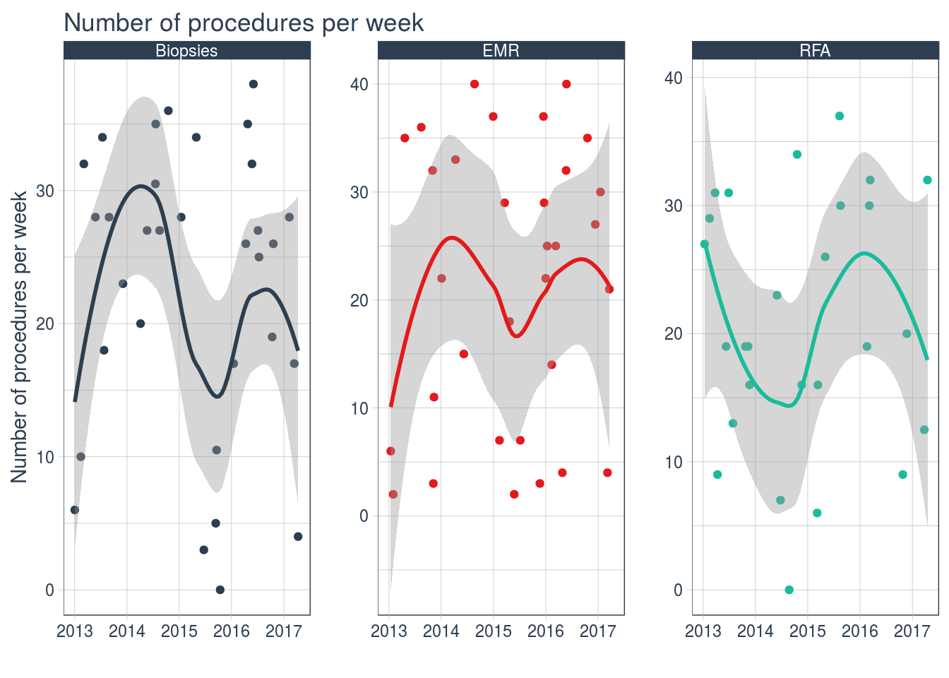
Predictions
Of course one of the best things about Time series analysis is the ability to forecast. We can use the aptly named forecast package to do this and an example can be seen here More detail about forecasting can be found here: http://a-little-book-of-r-for-time-series.readthedocs.io/en/latest/index.html including examples in R.